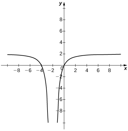
Refer Again to the Graph Figure 1 Select All True Statements About the Graph
2. Limits
2.ii The Limit of a Function
Learning Objectives
- Using correct notation, depict the limit of a function.
- Use a table of values to estimate the limit of a function or to identify when the limit does non exist.
- Use a graph to guess the limit of a part or to identify when the limit does non be.
- Define ane-sided limits and provide examples.
- Explain the relationship between one-sided and 2-sided limits.
- Using correct notation, depict an infinite limit.
- Define a vertical asymptote.
The concept of a limit or limiting process, essential to the agreement of calculus, has been around for thousands of years. In fact, early mathematicians used a limiting procedure to obtain better and ameliorate approximations of areas of circles. Yet, the formal definition of a limit—as we know and sympathize it today—did non appear until the late 19th century. We therefore begin our quest to understand limits, as our mathematical ancestors did, past using an intuitive approach. At the terminate of this chapter, armed with a conceptual understanding of limits, we examine the formal definition of a limit.
Nosotros begin our exploration of limits past taking a look at the graphs of the functions
 , and
, and 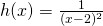 ,
,
which are shown in (Figure). In particular, let's focus our attention on the behavior of each graph at and effectually  .
.
Each of the three functions is undefined at , but if nosotros brand this statement and no other, we requite a very incomplete picture of how each function behaves in the vicinity of . To express the behavior of each graph in the vicinity of 2 more completely, we need to innovate the concept of a limit.
Intuitive Definition of a Limit
Permit's first take a closer look at how the function  behaves around in (Effigy). As the values of
  approach ii from either side of 2, the values of
  approach 4. Mathematically, nosotros say that the limit of
  equally approaches 2 is 4. Symbolically, we express this limit as
 .
.
From this very brief informal await at one limit, let's start to develop an intuitive definition of the limit. We can retrieve of the limit of a function at a number  equally being the one real number
  that the functional values approach as the -values approach , provided such a existent number exists. Stated more carefully, we accept the following definition:
We can estimate limits by constructing tables of functional values and past looking at their graphs. This process is described in the post-obit Trouble-Solving Strategy.
Problem-Solving Strategy: Evaluating a Limit Using a Table of Functional Values
- To evaluate
 , we begin by completing a table of functional values. We should cull 2 sets of -values—one set of values approaching and less than , and another set of values budgeted and greater than . (Effigy) demonstrates what your tables might look like.
Table of Functional Values for 





Use additional values equally necessary. Utilize boosted values every bit necessary. - Next, let'due south look at the values in each of the columns and determine whether the values seem to be budgeted a single value as we motion downwardly each column. In our columns, we look at the sequence
 and so on, and
  and then on. (Annotation: Although we accept chosen the -values
  , and and then forth, and these values will probably piece of work nearly every time, on very rare occasions nosotros may need to modify our choices.)
 - If both columns approach a common
 -value , we land
  . We can use the post-obit strategy to confirm the result obtained from the table or as an alternative method for estimating a limit.
 - Using a graphing estimator or computer software that allows us graph functions, we can plot the role , making sure the functional values of for -values most are in our window. We can use the trace feature to move along the graph of the function and sentry the -value readout equally the -values approach . If the -values approach equally our -values approach from both directions, then . We may need to zoom in on our graph and echo this process several times.
Nosotros employ this Problem-Solving Strategy to compute a limit in (Effigy).
Evaluating a Limit Using a Table of Functional Values 1
Evaluate  using a tabular array of functional values.
Evaluating a Limit Using a Table of Functional Values 2
Evaluate  using a table of functional values.
Estimate  using a table of functional values. Utilise a graph to ostend your estimate.
Solution
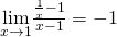
At this point, nosotros meet from (Effigy) and (Effigy) that information technology may be only every bit like shooting fish in a barrel, if not easier, to estimate a limit of a role by inspecting its graph equally it is to guess the limit past using a table of functional values. In (Effigy), we evaluate a limit exclusively by looking at a graph rather than by using a tabular array of functional values.
Evaluating a Limit Using a Graph
For  shown in (Effigy), evaluate
  .
.
Based on (Figure), we make the following observation: Information technology is possible for the limit of a function to be at a point, and for the function to exist defined at this point, just the limit of the role and the value of the function at the point may be different.
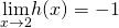
Utilize the graph of  in (Effigy) to evaluate
  , if possible.
Solution
 .
.
Looking at a table of functional values or looking at the graph of a function provides us with useful insight into the value of the limit of a part at a given point. However, these techniques rely too much on guesswork. Nosotros somewhen need to develop culling methods of evaluating limits. These new methods are more algebraic in nature and we explore them in the side by side department; however, at this indicate we introduce two special limits that are foundational to the techniques to come.
2 Of import Limits
Let be a real number and  be a constant.
We can brand the post-obit observations about these two limits.
- For the first limit, observe that every bit approaches , so does , because
 . Consequently,
  .
. - For the 2d limit, consider (Figure).
| |  | | | |
|---|---|---|---|---|
| | | | | |
| | | | | |
| | | | | |
| | | | |
Discover that for all values of (regardless of whether they are approaching ), the values remain constant at . We have no choice but to conclude  .
.
The Existence of a Limit
As we consider the limit in the next example, proceed in listen that for the limit of a part to be at a bespeak, the functional values must approach a single existent-number value at that bespeak. If the functional values do not arroyo a unmarried value, and then the limit does non be.
Evaluating a Limit That Fails to Exist
Evaluate  using a table of values.
Use a table of functional values to evaluate  , if possible.
Solution
does non exist.
One-Sided Limits
Sometimes indicating that the limit of a function fails to be at a signal does non provide u.s. with enough data about the behavior of the function at that particular betoken. To see this, we at present revisit the function  introduced at the beginning of the section (encounter (Figure)(b)). As we pick values of close to two, does not approach a single value, so the limit as approaches 2 does not exist—that is,
  DNE. Even so, this statement lone does not give united states a consummate flick of the beliefs of the function around the -value 2. To provide a more accurate clarification, we introduce the idea of a ane-sided limit. For all values to the left of 2 (or the negative side of 2),
  . Thus, as approaches 2 from the left, approaches −1. Mathematically, nosotros say that the limit equally approaches 2 from the left is −1. Symbolically, we express this idea as
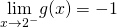 .
.
Similarly, equally approaches 2 from the correct (or from the positive side), approaches one. Symbolically, we express this thought as
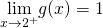 .
.
We tin now present an informal definition of ane-sided limits.
Evaluating One-Sided Limits
Utilise a table of functional values to guess the following limits, if possible.


Solution
a. 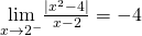 ; b.
; b. 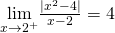
Let us now consider the relationship betwixt the limit of a function at a point and the limits from the right and left at that signal. It seems articulate that if the limit from the right and the limit from the left have a common value, then that common value is the limit of the function at that point. Similarly, if the limit from the left and the limit from the right accept on unlike values, the limit of the function does not exist. These conclusions are summarized in (Figure).
Space Limits
Evaluating the limit of a part at a point or evaluating the limit of a office from the right and left at a point helps u.s.a. to narrate the behavior of a office around a given value. Equally we shall see, we can also describe the behavior of functions that do non have finite limits.
We now turn our attention to  , the third and final role introduced at the first of this section (run across (Effigy)(c)). From its graph we run into that as the values of arroyo two, the values of become larger and larger and, in fact, become space. Mathematically, we say that the limit of as approaches ii is positive infinity. Symbolically, we express this thought as
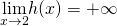 .
.
More more often than not, nosotros define infinite limits as follows:
It is important to understand that when we write statements such equally 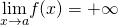 or
or 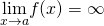 nosotros are describing the behavior of the function, every bit nosotros have but divers it. Nosotros are not asserting that a limit exists. For the limit of a role to exist at , it must approach a real number as approaches . That said, if, for example,
 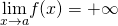 , nosotros always write rather than DNE.
Recognizing an Space Limit
It is useful to point out that functions of the form  , where
  is a positive integer, have infinite limits as approaches from either the left or right ((Figure)). These limits are summarized in (Effigy).
Infinite Limits from Positive Integers
If is a positive even integer, then
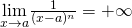 .
.
If is a positive odd integer, then
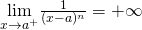
and
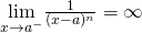 .
.
Nosotros should also indicate out that in the graphs of , points on the graph having -coordinates very most to are very close to the vertical line  . That is, every bit approaches , the points on the graph of are closer to the line . The line is called a vertical asymptote of the graph. We formally ascertain a vertical asymptote as follows:
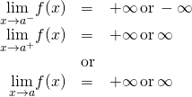
Definition
Permit exist a function. If any of the post-obit conditions concord, and then the line is a vertical asymptote of :
Finding a Vertical Asymptote
Solution
a. 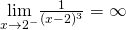 ;
;
b. 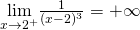 ;
;
c.  DNE. The line is the vertical asymptote of
  .
.
In the adjacent example we put our knowledge of various types of limits to use to analyze the behavior of a role at several different points.
Behavior of a Function at Dissimilar Points
Chapter Opener: Einstein'south Equation
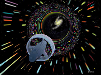
In the chapter opener we mentioned briefly how Albert Einstein showed that a limit exists to how fast any object can travel. Given Einstein's equation for the mass of a moving object, what is the value of this bound?
Solution
Our starting point is Einstein'southward equation for the mass of a moving object,
 ,
,
where  is the object's mass at rest,
  is its speed, and is the speed of light. To see how the mass changes at high speeds, we can graph the ratio of masses
  as a function of the ratio of speeds,
  ((Figure)).
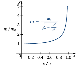
Nosotros can run across that as the ratio of speeds approaches 1—that is, every bit the speed of the object approaches the speed of light—the ratio of masses increases without spring. In other words, the function has a vertical asymptote at  . We tin can endeavor a few values of this ratio to test this idea.
 |  |  |
|---|---|---|
| 0.99 | 0.1411 | 7.089 |
| 0.999 | 0.0447 | 22.37 |
| 0.9999 | 0.0141 | 70.71 |
Thus, co-ordinate to (Figure), if an object with mass 100 kg is traveling at 0.9999, its mass becomes 7071 kg. Since no object can have an infinite mass, we conclude that no object can travel at or more than the speed of calorie-free.
Key Concepts
- A table of values or graph may be used to estimate a limit.
- If the limit of a function at a signal does not exist, it is still possible that the limits from the left and right at that signal may exist.
- If the limits of a function from the left and right be and are equal, then the limit of the function is that common value.
- We may use limits to describe infinite behavior of a role at a point.
Key Equations
For the following exercises, consider the office  .
.
2.What exercise your results in the preceding exercise indicate about the 2-sided limit  ? Explain your response.
Solution
does non exist because  .
.
For the following exercises, consider the function  .
.
4.What does the table of values in the preceding exercise bespeak about the function ?
Solution

5.To which mathematical abiding does the limit in the preceding practice appear to be getting closer?
In the following exercises, use the given values of to set up a tabular array to evaluate the limits. Round your solutions to eight decimal places.
Solution
a. 1.98669331; b. ane.99986667; c. 1.99999867; d. ane.99999999; e. 1.98669331; f. ane.99986667; m. 1.99999867; h. 1.99999999; 
8.Use the preceding two exercises to theorize (guess) the value of the following limit:  for , a positive real value.
Solution

In the post-obit exercises, set up a table of values to observe the indicated limit. Round to eight digits.
Solution
a. −0.80000000; b. −0.98000000; c. −0.99800000; d. −0.99980000; e. −1.2000000; f. −one.0200000; thousand. −1.0020000; h. −1.0002000;

Solution
a. −37.931934; b. −3377.9264; c. −333,777.93; d. −33,337,778; eastward. −29.032258; f. −3289.0365; g. −332,889.04; h. −33,328,889
Solution
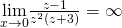
a. 0.13495277; b. 0.12594300; c. 0.12509381; d. 0.12500938; east. 0.11614402; f. 0.12406794; 1000. 0.12490631; h. 0.12499063;
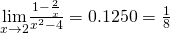
In the post-obit exercises, set up a table of values and round to eight meaning digits. Based on the tabular array of values, make a guess about what the limit is. Then, utilize a calculator to graph the function and decide the limit. Was the conjecture correct? If not, why does the method of tables neglect?
Solution
a. −10.00000; b. −100.00000; c. −1000.0000; d. −10,000.000; Guess: 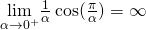 , Actual: DNE
![A graph of the function (1/alpha) * cos (pi / alpha), which oscillates gently until the interval [-.2, .2], where it oscillates rapidly, going to infinity and negative infinity as it approaches the y axis.](https://s3-us-west-2.amazonaws.com/courses-images/wp-content/uploads/sites/2332/2018/01/11202929/CNX_Calc_Figure_02_02_214.jpg)
In the following exercises, consider the graph of the office shown hither. Which of the statements about are truthful and which are faux? Explain why a argument is false.
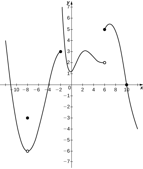
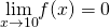
17. 
xviii. 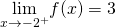
Solution
Imitation; 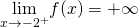
19. 
20. 
In the following exercises, utilise the following graph of the function to find the values, if possible. Gauge when necessary.
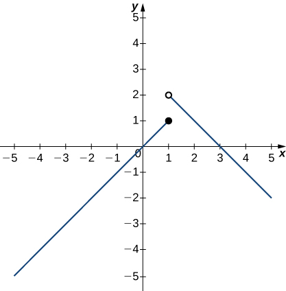 i. The first segment is linear with a slope of i and goes through the origin. Its endpoint is a closed circle at (1,1). The 2d segment is also linear with a slope of -one. It begins with the open circle at (i,2).">
21. 
22. 
23.
24. 
25. 
In the following exercises, use the graph of the office shown here to find the values, if possible. Estimate when necessary.

26. 
27. 
28. 
29.
In the following exercises, utilise the graph of the function shown here to notice the values, if possible. Estimate when necessary.
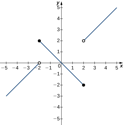 2, has a gradient of 1, and begins at the open circle (two,2).">
30. 
31. 
32. 
33. 
34. 
35.
In the following exercises, apply the graph of the function  shown hither to observe the values, if possible. Estimate when necessary.
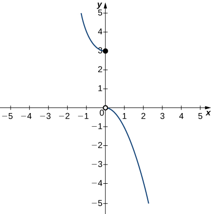 =0 and is the left half of an upward opening parabola with vertex at the airtight circle (0,iii). The second exists for ten>0 and is the correct half of a downward opening parabola with vertex at the open circumvolve (0,0).">
36. 
37. 
38. 
In the following exercises, apply the graph of the function  shown here to find the values, if possible. Approximate when necessary.
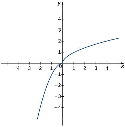
39. 
40. 
41. 
In the post-obit exercises, use the graph of the function shown here to detect the values, if possible. Gauge when necessary.
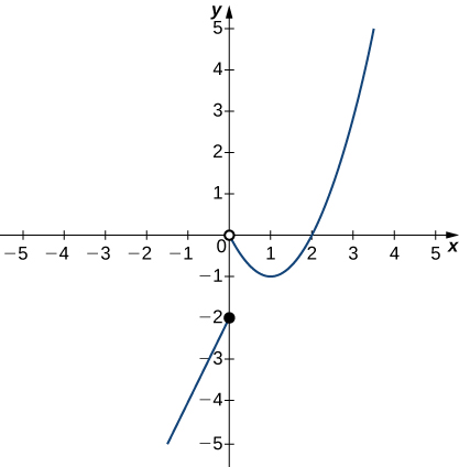 0, and there is a closed circle at the origin.">
42.
43.
44.
45.
46.
In the following exercises, sketch the graph of a office with the given properties.
47.  , the function is not defined at
  .
.
48.  ,
, 
Solution
Answers may vary.
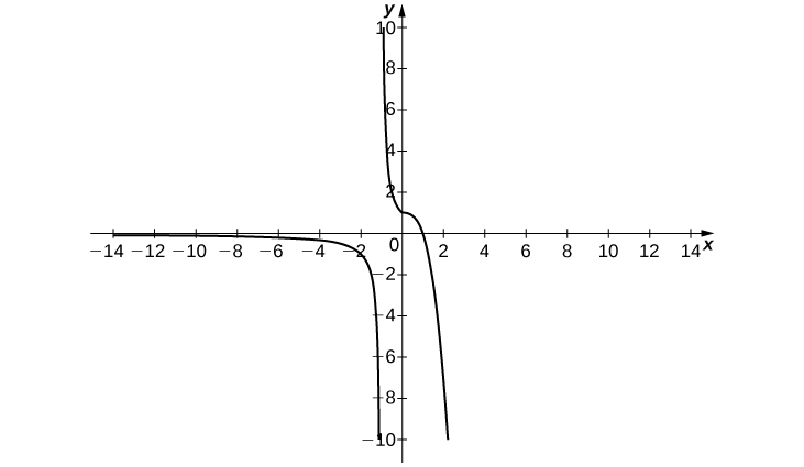
49.  ,
, 
50.  ,
,
Solution
Answers may vary.
51. 
floresunearithe55.blogspot.com
Source: https://opentextbc.ca/calculusv1openstax/chapter/the-limit-of-a-function/
0 Response to "Refer Again to the Graph Figure 1 Select All True Statements About the Graph"
Postar um comentário